LB-SPR tutorial

library(magrittr) # required for this vignette to work

1. Installing `lbmstoolbox` package

For this vigenette to work the lbmstoolbox package must be installed and exist in whatever R’s libpath of yours. To do so you can install it widely on the system by using devtools::install_github(..) or locally by renv::install. if ran interactively, ensure that the working directory is set to the vignettes folder - use setwd as suits you best.

2. Read sampling and biological data

A data sample has been provided to showcase how both algorithm interfaces work. The first element of the list is the catch’s length composition that the model will assess. This structure, in turn, stores two dataframes: i) a long one where years and lengths are laid as rows and ii) a wide one where years are set as columns and lengths as rows. Both dataframes contain MeanLength, the name of the column holding the length classes.

The second element is a list with the biological parameters of the species being evaluated, which we will call spp.demersal.

spp_sampling_details <- readRDS("data/spp_test_data.rds")

2.1 Showcase long dataframe

catch_data <- spp_sampling_details$catch_data
catch_data$long %>%
  head(6)
#>   year interval MeanLength catch
#> 1 2013    (3,4]        3.5     0
#> 2 2013    (4,5]        4.5     0
#> 3 2013    (5,6]        5.5     0
#> 4 2013    (6,7]        6.5     0
#> 5 2013    (7,8]        7.5     1
#> 6 2013    (8,9]        8.5     0

2.2 Showcase wide dataframe

catch_data$wide %>%
  head(6)
#>   MeanLength 2013 2014 2015 2016 2017 2018 2019 2020
#> 1        3.5    0    0    0    0    0    0    0    0
#> 2        4.5    0    0    0    0    0    0    0    0
#> 3        5.5    0    0    0    0    0    0    0    0
#> 4        6.5    0    0    0    0    0    0    0    0
#> 5        7.5    1    0    0    0    0    0    0    0
#> 6        8.5    0    0    0    0    0    0    0    0

2.3 Showcase wide dataframe

spp_sampling_details$bio_params
#> $linf
#> [1] 42.41
#> 
#> $k
#> [1] 0.21
#> 
#> $t0
#> [1] -1.202
#> 
#> $lwa
#> [1] 0.012
#> 
#> $lwb
#> [1] 3.011
#> 
#> $l50
#> [1] 19.45
#> 
#> $M
#> [1] 0.354
#> 
#> $max_age
#> [1] 9
#> 
#> $rec_variability_mean
#> [1] 0.748
#> 
#> $rec_variability_sd
#> [1] 0.293
#> 
#> $max_age
#> [1] 9
#> 
#> $fecb
#> [1] 3.011
#> 
#> $l95
#> [1] 22.37

3. Run LB-SPR

3.1 Build biological parameters required by LB-SPR

Please visit LBSPR documentation for further details. fecb defines the relationship between size and fecundity. By default, LB-SPR sets it to 3. We use the provided b exponent obtained from the weight-length relationship.

The biological parameters here provided contains the union of those required by LB-SPR and LIME. Let’s strip off LIME’s specific parameters and build LBSPR’S missing ones.

bio_params <- spp_sampling_details$bio_params

# We need to provide MK
bio_params$mk <- round(bio_params$M / bio_params$M, 2)
# ... And get rid of those that not required
bio_params$M <- NULL
bio_params$t0 <- NULL
bio_params$max_age <- NULL
bio_params$rec_variability_mean <- NULL
bio_params$rec_variability_sd <- NULL
bio_params
#> $linf
#> [1] 42.41
#> 
#> $k
#> [1] 0.21
#> 
#> $lwa
#> [1] 0.012
#> 
#> $lwb
#> [1] 3.011
#> 
#> $l50
#> [1] 19.45
#> 
#> $max_age
#> [1] 9
#> 
#> $fecb
#> [1] 3.011
#> 
#> $l95
#> [1] 22.37
#> 
#> $mk
#> [1] 1

3.2 Run LB-SPR

If LB-SPR is run with the flag simul set to TRUE, re-runs the simulation function to provide extra details for each time step used as follows:

Observed catch-at-length
Relative observed catch-at-length (each catch is divided by the maximum)
Standardised length structure of the underlying fished population
Standardised length structure of the underlying unfished population
Standardised estimated catch as a result of applying the estimated selectivity to the estimated fished population
Standardised estimated catch as a result of applying the estimated selectivity to the estimated unfished population

iim_lbspr <- lbmstoolbox::LbsprLbms$new(
  bio_params,
  catch_data
)
result_lbspr <- iim_lbspr$run(simul = TRUE)
#> A blank LB_pars object created
#> Default values have been set for some parameters
#> File not found. A blank LB_lengths object created
#> Fitting model
#> Year:
#> 1
#> 2
#> 3
#> 4
#> 5
#> 6
#> 7
#> 8
#> ngtg increased to 18 because of small bin size
#> ngtg increased to 18 because of small bin size
#> ngtg increased to 18 because of small bin size
#> ngtg increased to 18 because of small bin size
#> ngtg increased to 18 because of small bin size
#> ngtg increased to 18 because of small bin size
#> ngtg increased to 18 because of small bin size
#> ngtg increased to 18 because of small bin size

3.3 Breaking down results

Results are provided in two flavors: i) evaluation where estimates of the model are held and ii) simulation where the aforementioned extra details can be found. Within this section, also the raw output yielded by the simulation function are provided, should you be interested in doing more with it.

In addition, the estimate dataframe provides the confidence intervals of FM and SPR. These columns are prefixed by lower and upper, respectively.

3.3.1 Estimates dataframe

result_lbspr$evaluation$estimates %>%
  head(3)
#>    SL50  SL95   FM  SPR years lower_spr upper_spr lower_fm upper_fm
#> 1 17.37 20.44 2.68 0.12  2013 0.1086088 0.1313912 2.506141 2.853859
#> 2 17.38 20.48 2.72 0.12  2014 0.1030489 0.1369511 2.394831 3.045169
#> 3 17.37 20.41 2.75 0.12  2015 0.1068953 0.1331047 2.426899 3.073101

3.3.2 Simulation dataframes

Below an example of the simulation dataframe for one single time step. The relevant columns are:

unfished_pop: length structure of the unfished population.
fished_pop: length structure of the fished population.
unfished_vul: estimated catch yielded by the estimated unfished population and selectivity.
expected_catch: estimated catch yielded by the estimated fished population and selectivity.
real_catch: observed catch in absolute numbers
relative_catch: Relative-to-maximum observed catch

result_lbspr$simulation$model_info %>%
  head(3)
#>   year lengths unfished_pop fished_pop unfished_vul    exp_catch real_catch
#> 1 2013     3.5   0.02593895 0.04597458            0 2.231862e-07          0
#> 2 2013     4.5   0.02593895 0.04597458            0 5.823691e-07          0
#> 3 2013     5.5   0.02593895 0.04597458            0 1.519593e-06          0
#>   relative_catch
#> 1              0
#> 2              0
#> 3              0

4. Plot examples

4.1 Estimates plot

A quick example on how to plot SPR and its confidence interval is shown below.

estimates <- result_lbspr$evaluation$estimates
g <- estimates %>%
  ggplot2::ggplot(ggplot2::aes(x = years, y = SPR)) +
  ggplot2::geom_point() +
  ggplot2::geom_line() +
  ggplot2::geom_ribbon(ggplot2::aes(x = years, ymin = lower_spr, ymax = upper_spr, fill = "maroon2", alpha = 0.1)) +
  ggplot2::theme_bw() +
  ggplot2::theme(legend.position = "none")

g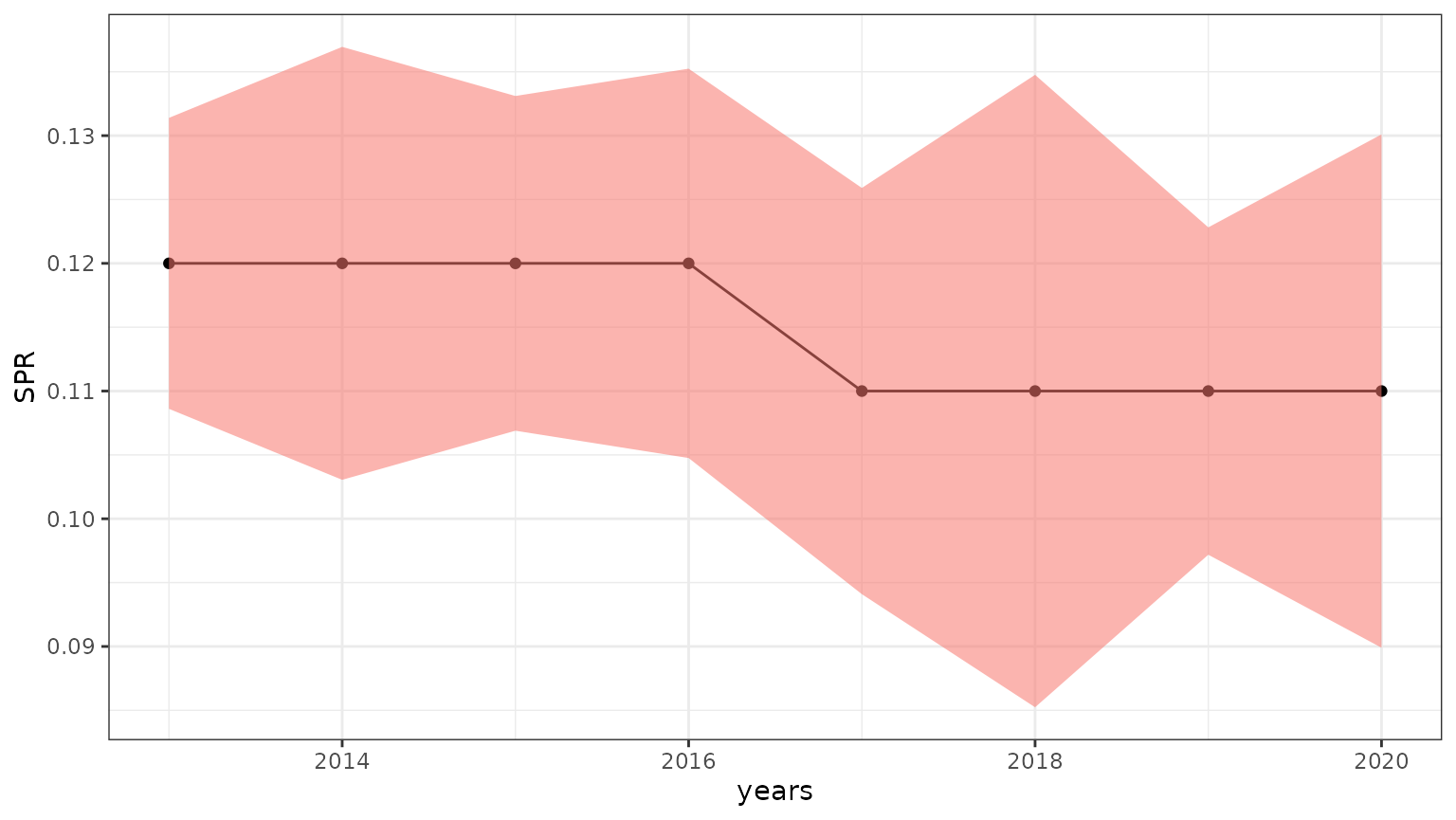

4.2 Simulation plot

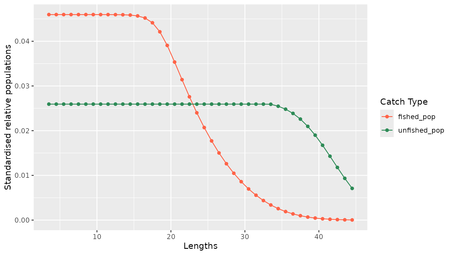
Below two different plots are displayed. The first one shows the estimated catch from both the estimated fished and unfished length structured for year 2015. The second one plots the estimated fished and unfished populations for the same year.

4.2.1 Estimated catch

catch_2015 <- result_lbspr$simulation$model_info %>%
  dplyr::filter(year == 2015) %>%
  dplyr::select(lengths, unfished_vul, exp_catch) %>%
  tidyr::pivot_longer(!lengths, names_to = "variables", values_to = "values")

g <- catch_2015 %>%
  ggplot2::ggplot(ggplot2::aes(x = lengths, y = values, color = variables)) +
  ggplot2::geom_point() +
  ggplot2::geom_line() +
  ggplot2::xlab("Lengths") +
  ggplot2::ylab("Standardised relative catch") +
  ggplot2::scale_color_manual(
    name = "Catch Type",
    values = c(
      unfished_vul = "seagreen",
      exp_catch = "tomato"
    )
  )

g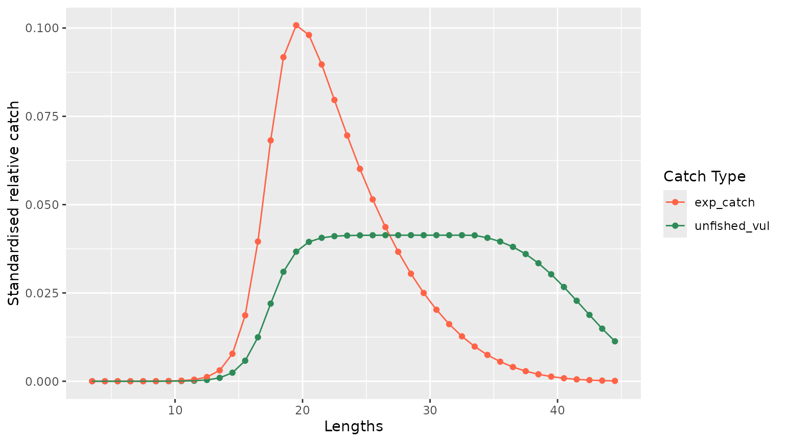

4.2.1 Estimated populations

population_2015 <- result_lbspr$simulation$model_info %>%
  dplyr::filter(year == 2015) %>%
  dplyr::select(lengths, unfished_pop, fished_pop) %>%
  tidyr::pivot_longer(!lengths, names_to = "variables", values_to = "values")

g <- population_2015 %>%
  ggplot2::ggplot(ggplot2::aes(x = lengths, y = values, color = variables)) +
  ggplot2::geom_point() +
  ggplot2::geom_line() +
  ggplot2::xlab("Lengths") +
  ggplot2::ylab("Standardised relative populations") +
  ggplot2::scale_color_manual(
    name = "Catch Type",
    values = c(
      unfished_pop = "seagreen",
      fished_pop = "tomato"
    )
  )

g

1. Installing lbmstoolbox package